Code
library(tidyverse)
library(scales)
library(glue)
library(ggrepel)
library(showtext)
library(colorspace)
library(forcats)The WHO Global Health Expenditure Database (GHED) makes it possible to compare how countries pay for care: public schemes, voluntary insurance, and household out-of-pocket spending, alongside what the money buys (curative vs preventive care, and more). This notebook uses the TidyTuesday 2026-04-21 release (WHO GHED via ONE Data).
library(tidyverse)
library(scales)
library(glue)
library(ggrepel)
library(showtext)
library(colorspace)
library(forcats)data_dir <- file.path(getwd(), "data")
che <- readr::read_csv(
file.path(data_dir, "health_spending.csv"),
show_col_types = FALSE
)
fin <- readr::read_csv(
file.path(data_dir, "financing_schemes.csv"),
show_col_types = FALSE
)
pur <- readr::read_csv(
file.path(data_dir, "spending_purpose.csv"),
show_col_types = FALSE
)NOTE_TEXT <- "2023 cross-section where available; GHED units per TidyTuesday dictionary"
SOURCE_TEXT <- "TidyTuesday 2026-04-21 / WHO GHED (via ONE Data)"
CAPTION <- glue("Note: {NOTE_TEXT} | Source: {SOURCE_TEXT} | \u00A9 2026 chokotto")
theme_fm <- theme_minimal(base_size = 12) +
theme(
plot.background = element_rect(fill = "white", color = NA),
panel.background = element_rect(fill = "#f8fafc", color = NA),
panel.grid.major = element_line(color = "#e2e8f0", linewidth = 0.3),
panel.grid.minor = element_blank(),
text = element_text(color = "#334155"),
axis.text = element_text(color = "#475569"),
plot.title = element_text(color = "#1e293b", face = "bold", size = 14),
plot.subtitle = element_text(color = "#64748b", size = 10),
plot.caption = element_text(
face = "italic", color = "#94a3b8", size = 9,
hjust = 0, margin = margin(t = 12)
),
plot.caption.position = "plot",
legend.background = element_rect(fill = "white", color = NA),
plot.margin = margin(15, 15, 15, 15)
)
COL_GOV <- "#0284c7"
COL_OOP <- "#dc2626"
COL_CUR <- "#0d9488"
COL_PRV <- "#f59e0b"che_23 <- che |>
filter(
year == 2023,
expenditure_type == "Current Health Expenditure (CHE)",
unit == "constant 2023 US$"
)
top15 <- che_23 |>
slice_max(order_by = value, n = 15) |>
mutate(
country_name = fct_reorder(country_name, value),
dollar_billions = value / 1e9
)
format_usd_trillions <- function(x) {
paste0("$", scales::comma(x / 1000, accuracy = 0.1), "T")
}
ggplot(top15, aes(x = dollar_billions, y = country_name)) +
geom_segment(
aes(x = 0, xend = dollar_billions, yend = country_name),
color = "#e2e8f0", linewidth = 0.9
) +
geom_point(color = COL_GOV, size = 4.5) +
geom_text(
aes(label = dollar(value, scale = 1e-9, accuracy = 0.1, suffix = "B")),
hjust = -0.15, size = 3.2, color = "#475569"
) +
scale_x_continuous(
labels = format_usd_trillions,
breaks = scales::breaks_extended(n = 5),
expand = expansion(mult = c(0, 0.08))
) +
labs(
title = "Fifteen largest national health budgets (CHE, constant 2023 US$)",
subtitle = "Current health expenditure aggregates all financing sources | Year 2023",
x = "Current health expenditure (USD, trillions)",
y = NULL,
caption = CAPTION
) +
theme_fm +
theme(panel.grid.major.y = element_blank())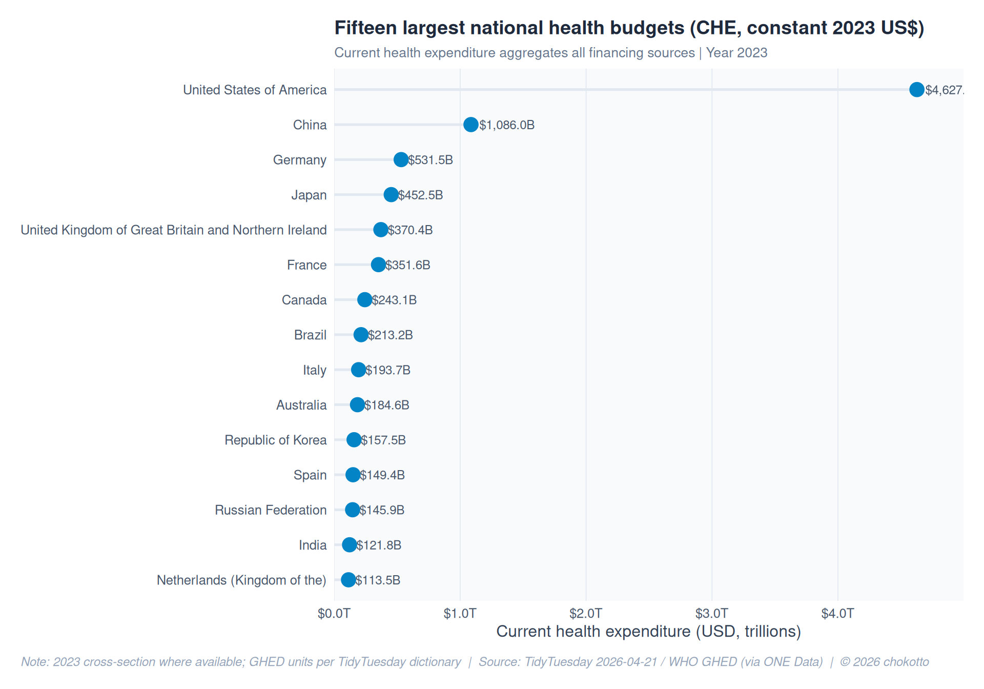
fin_pct <- fin |>
  filter(
    year == 2023,
    unit == "% of current health expenditure"
  ) |>
  mutate(
    scheme_short = case_when(
      str_detect(financing_scheme, "Government schemes") ~ "Government",
      str_detect(financing_scheme, "out-of-pocket") ~ "Out_of_pocket",
      str_detect(financing_scheme, "Voluntary") ~ "Voluntary",
      TRUE ~ NA_character_
    )
  ) |>
  filter(!is.na(scheme_short)) |>
  group_by(country_name, scheme_short) |>
  summarise(value = sum(value, na.rm = TRUE), .groups = "drop") |>
  pivot_wider(names_from = scheme_short, values_from = value)

fin_plot <- fin_pct |>
  inner_join(
    che_23 |>
      select(country_name, che_usd = value) |>
      slice_max(che_usd, n = 60),
    by = "country_name"
  ) |>
  filter(!is.na(Government), !is.na(Out_of_pocket))

ggplot(fin_plot, aes(x = Government, y = Out_of_pocket)) +
  geom_point(aes(size = che_usd), alpha = 0.55, color = COL_GOV) +
  geom_smooth(
    method = "lm", se = FALSE, linewidth = 0.4,
    color = "#94a3b8", linetype = "dashed"
  ) +
  geom_text_repel(
    data = fin_plot |> slice_max(che_usd, n = 12),
    aes(label = country_name),
    size = 3, max.overlaps = 20,
    segment.color = "#e2e8f0"
  ) +
  scale_size_continuous(range = c(2, 10), labels = label_dollar(scale = 1e9, suffix = "B")) +
  scale_x_continuous(labels = label_number(suffix = "%")) +
  scale_y_continuous(labels = label_number(suffix = "%")) +
  labs(
    title = "Public compulsory financing vs household out-of-pocket (% of CHE)",
    subtitle = "Bubble size = total CHE (2023) | Labels: top 12 spenders among plotted countries",
    x = "Government & compulsory schemes (% of CHE)",
    y = "Household out-of-pocket (% of CHE)",
    size = "CHE (USD)",
    caption = CAPTION
  ) +
  theme_fm +
  theme(legend.position = "bottom")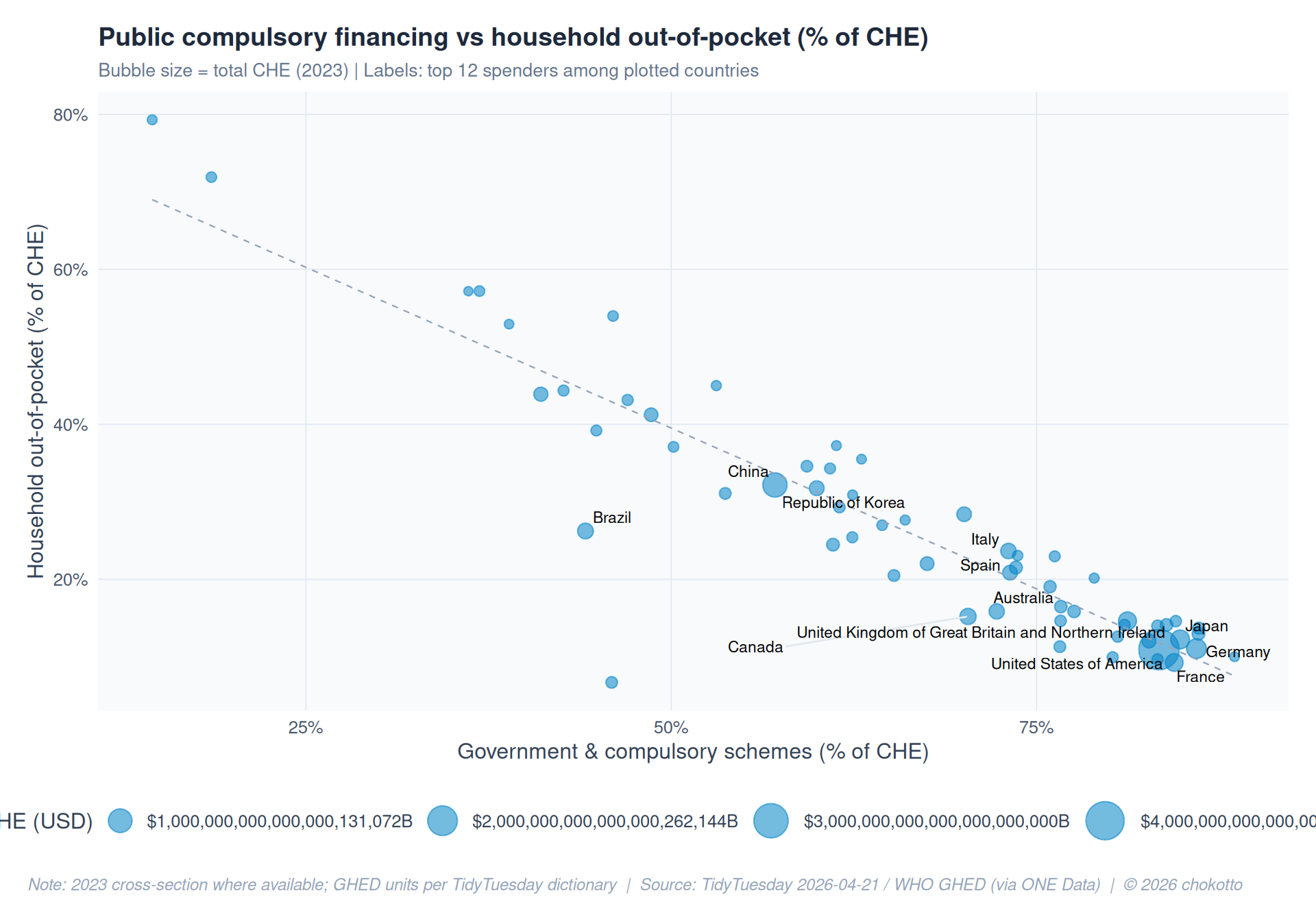
pur_23 <- pur |>
  filter(
    year == 2023,
    unit == "% of current health expenditure",
    spending_purpose %in% c("Curative care", "Preventive care")
  )

lv <- levels(top15$country_name)

cp <- pur_23 |>
  filter(country_name %in% lv) |>
  mutate(
    country_name = factor(country_name, levels = rev(lv)),
    spending_purpose = fct_relevel(spending_purpose, "Preventive care", "Curative care")
  )

ggplot(cp, aes(x = country_name, y = value, fill = spending_purpose)) +
  geom_col(position = position_dodge(width = 0.8), width = 0.72) +
  coord_flip() +
  scale_fill_manual(
    values = c("Curative care" = COL_CUR, "Preventive care" = COL_PRV)
  ) +
  scale_y_continuous(labels = label_number(suffix = "%")) +
  labs(
    title = "Curative vs preventive care as a share of CHE",
    subtitle = "Same 15 countries as the CHE ranking | 2023 | each bar is % of CHE (other functions omitted)",
    x = NULL,
    y = "Percent of current health expenditure",
    fill = NULL,
    caption = CAPTION
  ) +
  theme_fm +
  theme(legend.position = "top")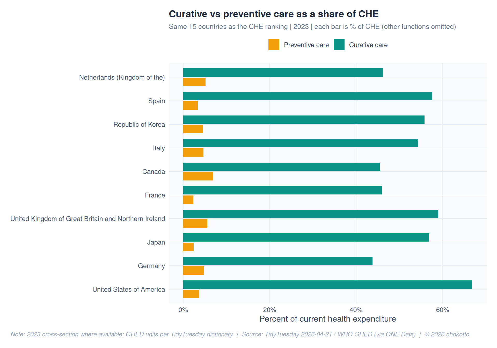
This post is part of TidyTuesday, a weekly data project.