TidyTuesday: Italian industrial production (ISTAT)

Beer, textiles, and shipbuilding in Italy: 150 years of official industrial production series from ISTAT (food & beverages, textiles, transport)

Overview

ISTAT publishes harmonised long series for Italian industry. This notebook uses the TidyTuesday 2026-05-05 release (readme): food_beverages.csv, textiles.csv, and transport.csv.

• Angles: how beer production recovered from wartime disruption; how cotton yarn climbed through industrialisation; how ships launched and average tonnage per ship evolved as shipyards scaled up.

Dataset

Analysis

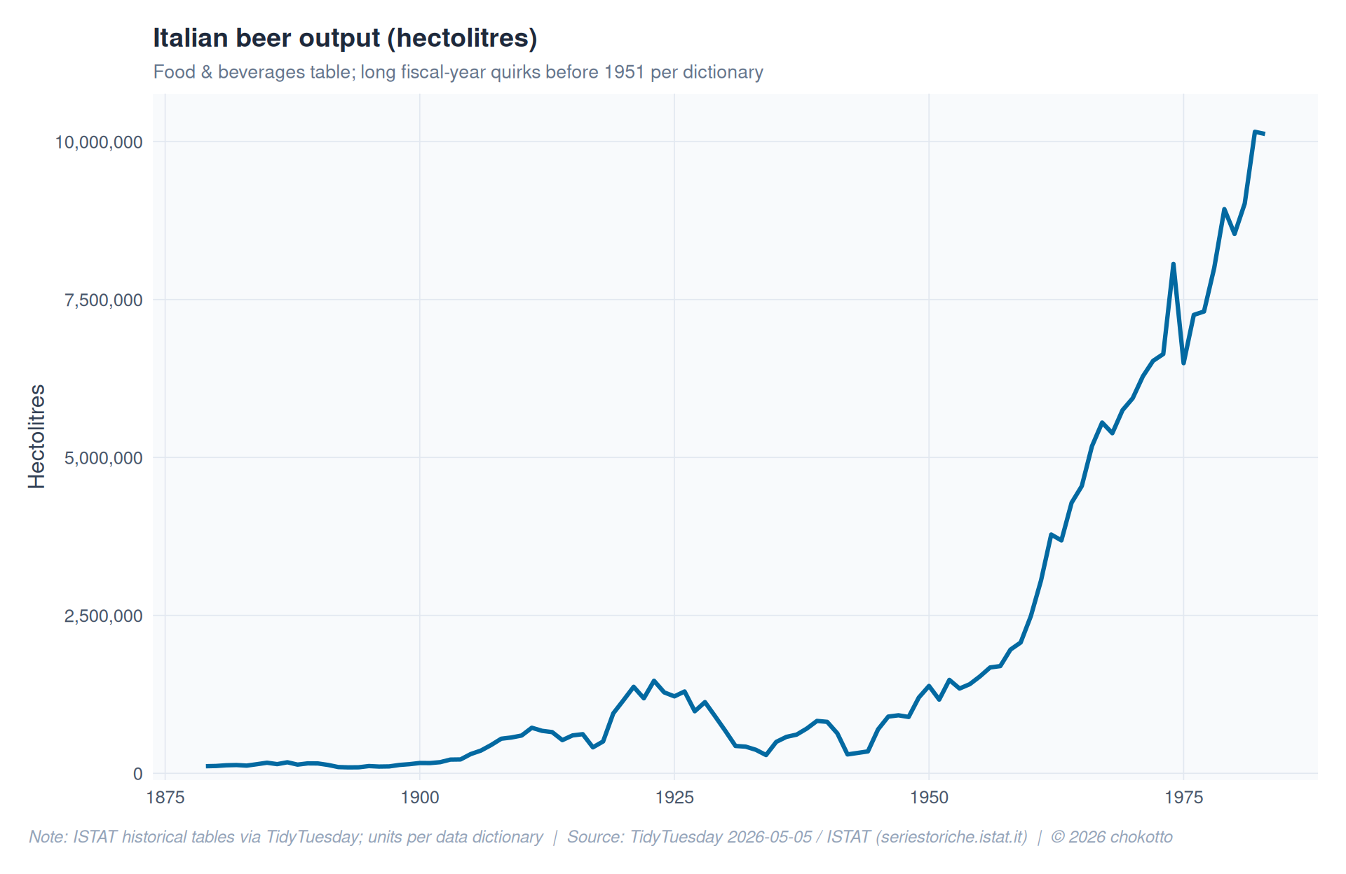
Beer production: shocks and recovery

beer <- food |>
  dplyr::filter(!is.na(Beer)) |>
  dplyr::select(Year, Beer)

ggplot(beer, aes(x = Year, y = Beer)) +
  geom_line(color = COL_BEER, linewidth = 1.1) +
  scale_y_continuous(
    labels = label_comma(),
    expand = expansion(mult = c(0.02, 0.06))
  ) +
  labs(
    title = "Italian beer output (hectolitres)",
    subtitle = "Food & beverages table; long fiscal-year quirks before 1951 per dictionary",
    x = NULL,
    y = "Hectolitres",
    caption = CAPTION
  ) +
  theme_fm

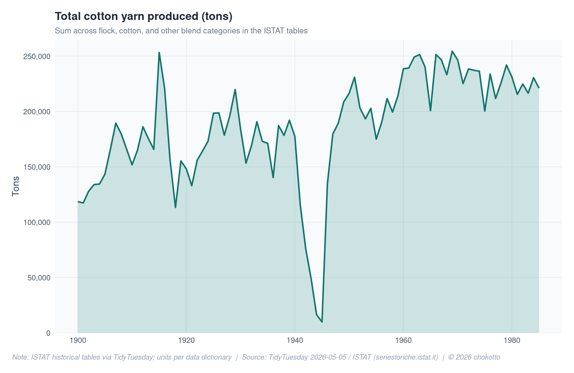
Cotton yarn: climb and late-century retrenchment

yarn <- tex |>
  dplyr::filter(!is.na(Total_yarn)) |>
  dplyr::select(Year, Total_yarn)

ggplot(yarn, aes(x = Year, y = Total_yarn)) +
  geom_area(fill = alpha(COL_YARN, 0.18), color = COL_YARN, linewidth = 0.9) +
  scale_y_continuous(labels = label_comma(), expand = expansion(mult = c(0, 0.04))) +
  labs(
    title = "Total cotton yarn produced (tons)",
    subtitle = "Sum across flock, cotton, and other blend categories in the ISTAT tables",
    x = NULL,
    y = "Tons",
    caption = CAPTION
  ) +
  theme_fm

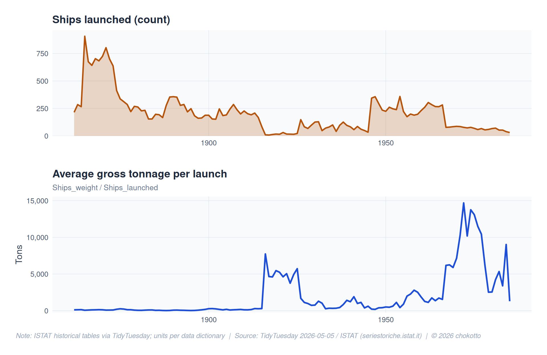
Ship launches and average gross tonnage

ships <- tr |>
  dplyr::filter(!is.na(Ships_launched), !is.na(Ships_weight), Ships_launched > 0) |>
  dplyr::mutate(avg_tonnage = Ships_weight / Ships_launched)

p1 <- ggplot(ships, aes(x = Year, y = Ships_launched)) +
  geom_area(fill = alpha(COL_SHIPS, 0.22), color = COL_SHIPS, linewidth = 0.9) +
  scale_y_continuous(labels = label_comma(), expand = expansion(mult = c(0, 0.06))) +
  labs(
    title = "Ships launched (count)",
    x = NULL,
    y = NULL
  ) +
  theme_fm +
  theme(plot.caption = element_blank())

p2 <- ggplot(ships, aes(x = Year, y = avg_tonnage)) +
  geom_line(color = "#1d4ed8", linewidth = 1) +
  scale_y_continuous(labels = label_comma(), expand = expansion(mult = c(0.02, 0.06))) +
  labs(
    title = "Average gross tonnage per launch",
    subtitle = "Ships_weight / Ships_launched",
    x = NULL,
    y = "Tons",
    caption = CAPTION
  ) +
  theme_fm

p1 / p2 + patchwork::plot_layout(heights = c(1, 1.1))

Key findings

• Beer shows sharp mid-century dislocation, then steady expansion from roughly the 1960s onward under a modern fiscal-year reporting regime.
• Cotton yarn rises across the 19th and 20th centuries, then contracts as supply chains and fibre mix shift.
• Shipbuilding moves from many small launches to fewer but heavier ships - average tonnage trends upward even when launch counts are volatile.

---

This post is part of the TidyTuesday project.

CautionDisclaimer

This analysis is for educational and practice purposes only. Data visualizations and interpretations are based on the provided dataset and may not represent complete or current information.