TidyTuesday: Mapping the global city link network (Wikidata Q-IDs)

TidyTuesday 2026-05-12 city links: mapping 5,470 cities and 10,596 edges from Wikidata Q-IDs

Overview

This week’s dataset comes as two tidy files that form a simple spatial network of cities. See the data notes and context in the TidyTuesday readme: https://github.com/rfordatascience/tidytuesday/blob/main/data/2026/2026-05-12/readme.md. The nodes live in cities.csv (5,470 rows) with Wikidata Q-IDs, names, country and continent labels, plus latitude/longitude. The edges live in links.csv (10,596 pairs) connecting Q-ID to Q-ID.

I’ll treat the pairs as city-to-city links and focus on what the global footprint looks like when we place every node on the map and draw the connections. The coordinates span longitudes from -172 to 178 and latitudes from -54.8 to 72.8, so coverage is truly global. A small amount of metadata is incomplete (countrycd is missing for 7 cities), but continent is present for all rows, which is handy for coloring or faceting. The angle here: build a lightweight world network view, then peek at basic structure—components and degrees—before settling on a readable map-first visualization.

Dataset

library(tidyverse)
library(ggplot2)
library(scales)
library(glue)
library(patchwork)

# Load this week's data
# tuesdata <- tidytuesdayR::tt_load('2026-05-12')

# Source/Note caption (Note | Source | copyright)
SOURCE_CAPTION <- "Note: Lng/lat are decimal degrees; links are Q-ID pairs joined to city coordinates  |  Source: TidyTuesday 2026-05-12 / rfordatascience (see readme)  |  \u00A9 2026 chokotto"

# Combined panel title / subtitle (filled in by weekly_dataviz.py / AI writer)
combined_title <- "A world map of 10,596 city links"
combined_subtitle <- "5,470 cities positioned by lat/lng; edges drawn between linked Q-ID pairs"

# --- Style mode: "figmamake" (light) or "dark" ---
STYLE_MODE <- "figmamake"

# FigmaMake style (light, clean, MM-aligned)
theme_fm <- theme_minimal(base_size = 12) +
  theme(
    plot.background = element_rect(fill = "white", color = NA),
    panel.background = element_rect(fill = "#f8fafc", color = NA),
    panel.grid.major = element_line(color = "#e2e8f0", linewidth = 0.3),
    panel.grid.minor = element_blank(),
    text = element_text(color = "#334155"),
    axis.text = element_text(color = "#475569"),
    plot.title = element_text(color = "#1e293b", face = "bold", size = 14),
    plot.subtitle = element_text(color = "#64748b", size = 10),
    plot.caption = element_text(
      face = "italic", color = "#94a3b8", size = 9,
      hjust = 0, margin = margin(t = 12)
    ),
    plot.caption.position = "plot",
    strip.text = element_text(color = "#1e293b", face = "bold"),
    legend.background = element_rect(fill = "white", color = NA),
    legend.text = element_text(color = "#475569"),
    plot.margin = margin(15, 15, 15, 15)
  )

# Dark style (kept for future mode switching)
# theme_dark_cap <- theme_minimal(base_size = 12) +
#   theme(
#     plot.background = element_rect(fill = "#0f172a", color = NA),
#     panel.background = element_rect(fill = "#0f172a", color = NA),
#     panel.grid.major = element_line(color = "#1e293b", linewidth = 0.3),
#     panel.grid.minor = element_blank(),
#     text = element_text(color = "#e2e8f0"),
#     axis.text = element_text(color = "#94a3b8"),
#     plot.title = element_text(color = "#f8fafc", face = "bold", size = 14),
#     plot.subtitle = element_text(color = "#94a3b8", size = 10),
#     plot.caption = element_text(
#       face = "italic", color = "#64748b", size = 9,
#       hjust = 0, margin = margin(t = 12)
#     ),
#     plot.caption.position = "plot",
#     strip.text = element_text(color = "#e2e8f0", face = "bold"),
#     legend.background = element_rect(fill = "#0f172a", color = NA),
#     legend.text = element_text(color = "#cbd5e1"),
#     plot.margin = margin(15, 15, 15, 15)
#   )

theme_active <- theme_fm  # switch: if (STYLE_MODE == "dark") theme_dark_cap else theme_fm

Exploratory Analysis

I start by reading both CSVs, validating IDs, and checking for missing metadata. Then I join city coordinates onto both ends of each link so we can plot great-circle-ish curves in ggplot2. A quick pass on components and degree counts will highlight hubs and isolates, and guide small design choices like edge alpha and node size for a legible, not-too-hairy world map

Visualization

cities <- readr::read_csv("data/cities.csv", show_col_types = FALSE)
links <- readr::read_csv("data/links.csv", show_col_types = FALSE)

# degree (hub) counts per city
degree_tbl <- dplyr::bind_rows(
  links %>% dplyr::transmute(id = source),
  links %>% dplyr::transmute(id = target)
) %>%
  dplyr::count(id, name = "degree")

cities_nodes <- cities %>%
  dplyr::left_join(degree_tbl, by = "id") %>%
  dplyr::mutate(degree = tidyr::replace_na(degree, 0),
                size_plot = pmin(degree, 30) + 0.5) # cap for visual scaling

# join coordinates to both ends of each link
links_coords <- links %>%
  dplyr::left_join(cities %>% dplyr::select(id, lng, lat), by = c("source" = "id")) %>%
  dplyr::rename(src_lng = lng, src_lat = lat) %>%
  dplyr::left_join(cities %>% dplyr::select(id, lng, lat), by = c("target" = "id")) %>%
  dplyr::rename(tgt_lng = lng, tgt_lat = lat) %>%
  dplyr::filter(!is.na(src_lat) & !is.na(tgt_lat))

# small set of top hubs to label
top_hubs <- cities_nodes %>%
  dplyr::filter(!is.na(lat) & !is.na(lng)) %>%
  dplyr::arrange(dplyr::desc(degree)) %>%
  dplyr::slice_head(n = 6)

# plot: edges first (low alpha), then nodes sized by degree, then a few labels
p <- ggplot() +
  geom_curve(
    data = links_coords,
    mapping = aes(x = src_lng, y = src_lat, xend = tgt_lng, yend = tgt_lat),
    curvature = 0.2,
    color = "#2f2f2f",
    alpha = 0.06,
    linewidth = 0.25
  ) +
  geom_point(
    data = cities_nodes %>% dplyr::filter(!is.na(lat) & !is.na(lng)),
    mapping = aes(x = lng, y = lat, size = size_plot),
    color = "#0b4471",
    alpha = 0.9
  ) +
  scale_size_continuous(range = c(0.6, 5), guide = "none") +
  geom_text(
    data = top_hubs,
    mapping = aes(x = lng, y = lat, label = name),
    size = 3.2,
    nudge_y = 1.2,
    color = "#111111"
  ) +
  coord_quickmap(expand = FALSE) +
  labs(title = combined_title,
       subtitle = combined_subtitle,
       x = NULL,
       y = NULL,
       caption = SOURCE_CAPTION) +
  theme_active

p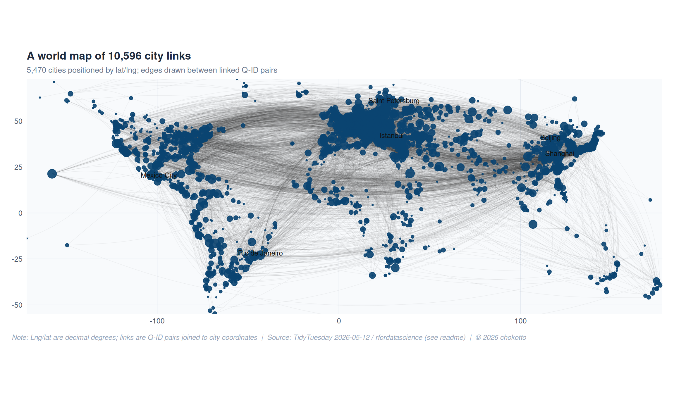

Key Findings

• The dataset lists 5,470 cities in cities.csv and 10,596 source–target links in links.csv
• City coordinates range from longitude -172 to 178 and latitude -54.8 to 72.8 (cities.csv)
• In the head, Fukaya (Q734532, Japan/Asia) appears, and the first link pairs Q734532 with Q873835; countrycd is missing in 7 of 5,470 rows

---

This post is part of the TidyTuesday weekly data visualization project.

CautionDisclaimer

This analysis is for educational and practice purposes only. Data visualizations and interpretations are based on the provided dataset and may not represent complete or current information.