TidyTuesday: Game adaptations on screen: budgets, box office, and scores

Exploring TidyTuesday’s game_films: theatrical video game adaptations, their budgets, grosses, and critic scores

Overview

This week’s dataset comes from the TidyTuesday release for 2026-06-09. See the readme for context and data dictionary. The single table, game_films.csv (439 rows, 20 columns), spans theatrical releases and other categories, with fields for title, director, release_date, box office (currency + totals), critic scores (Rotten Tomatoes and Metacritic), CinemaScore, distributors, and original game publishers.

Coverage varies by field: 96 rows include worldwide_box_office, 73 have Rotten Tomatoes, 63 have Metacritic, and 51 have CinemaScore. Budgets are often given as low/high ranges (with a currency code, frequently “$”). Domestic box office appears as strings that may include non-USD symbols (e.g., “¥790,000,000”). For this post, I focus on theatrical releases with available USD budgets and worldwide grosses to look at the money-vs-reception story for video game adaptations.

Dataset

library(tidyverse)   # ggplot2, dplyr, tidyr, readr, purrr, stringr, lubridate, forcats
library(scales)      # comma, dollar, label_number, cut_short_scale, percent
library(glue)        # glue("...")
library(broom)       # tidy() / glance() / augment() — wrap stat results into tibbles
library(patchwork)   # plot composition (p1 / p2, p1 + p2, etc.)
library(ggrepel)     # geom_text_repel / geom_label_repel — non-overlapping labels
library(gghighlight) # gghighlight() — focus selected series, fade the rest
library(ggdist)      # stat_halfeye() / stat_dots() / stat_lineribbon() — uncertainty viz
library(mgcv)        # gam() — backs geom_smooth(method = "gam")
library(tidymodels)  # rsample / parsnip / recipes / yardstick / broom — modeling tidyverse
library(sysfonts)
library(showtext)
showtext_auto()

# Per-file loads emitted by AI writer's main-viz block, which calls
# `read_csv("data/<name>.csv")` directly. This block is intentionally minimal —
# concrete CSV reads belong in `main-viz` so the chunk owns its dependencies.
data_dir <- "data"

# Source/Note caption (Note | Source | copyright)
SOURCE_CAPTION <- "Note: Box office/budgets as listed; currencies per fields; critic scores 0–100 where given  |  Source: TidyTuesday 2026-06-09 / game_films.csv (see readme for data sources)  |  © 2026 chokotto"

# Combined panel title / subtitle (filled in by weekly_dataviz.py / AI writer)
combined_title    <- "Video game films: money vs critics"
combined_subtitle <- "Theatrical releases with $ budgets and worldwide gross; point color shows critic score"

# --- FigmaMake palette (light, MM/TT shared) ---
FM_BG       <- "white"
FM_PANEL    <- "#f8fafc"
FM_GRID     <- "#e2e8f0"
FM_TEXT     <- "#334155"
FM_AXIS     <- "#475569"
FM_TITLE    <- "#1e293b"
FM_SUB      <- "#64748b"
FM_CAPTION  <- "#94a3b8"

# Discrete categorical palette — 8 hand-picked colors (R is 1-indexed: PAL[1]…PAL[8])
PAL <- c("#0369a1", "#7c3aed", "#16a34a", "#dc2626",
         "#ea580c", "#ca8a04", "#0891b2", "#9333ea")

theme_active <- theme_minimal(base_size = 12) +
  theme(
    plot.background   = element_rect(fill = FM_BG,    color = NA),
    panel.background  = element_rect(fill = FM_PANEL, color = NA),
    panel.grid.major  = element_line(color = FM_GRID, linewidth = 0.3),
    panel.grid.minor  = element_blank(),
    text              = element_text(color = FM_TEXT),
    axis.text         = element_text(color = FM_AXIS),
    plot.title        = element_text(color = FM_TITLE, face = "bold", size = 14),
    plot.subtitle     = element_text(color = FM_SUB,   size = 10),
    plot.caption      = element_text(face = "italic", color = FM_CAPTION, size = 9,
                                      hjust = 0, margin = margin(t = 12)),
    strip.text        = element_text(color = FM_TITLE, face = "bold"),
    legend.background = element_rect(fill = FM_BG, color = NA),
    legend.text       = element_text(color = FM_AXIS),
    plot.margin       = margin(t = 8, r = 12, b = 8, l = 12)
  )

Exploratory Analysis

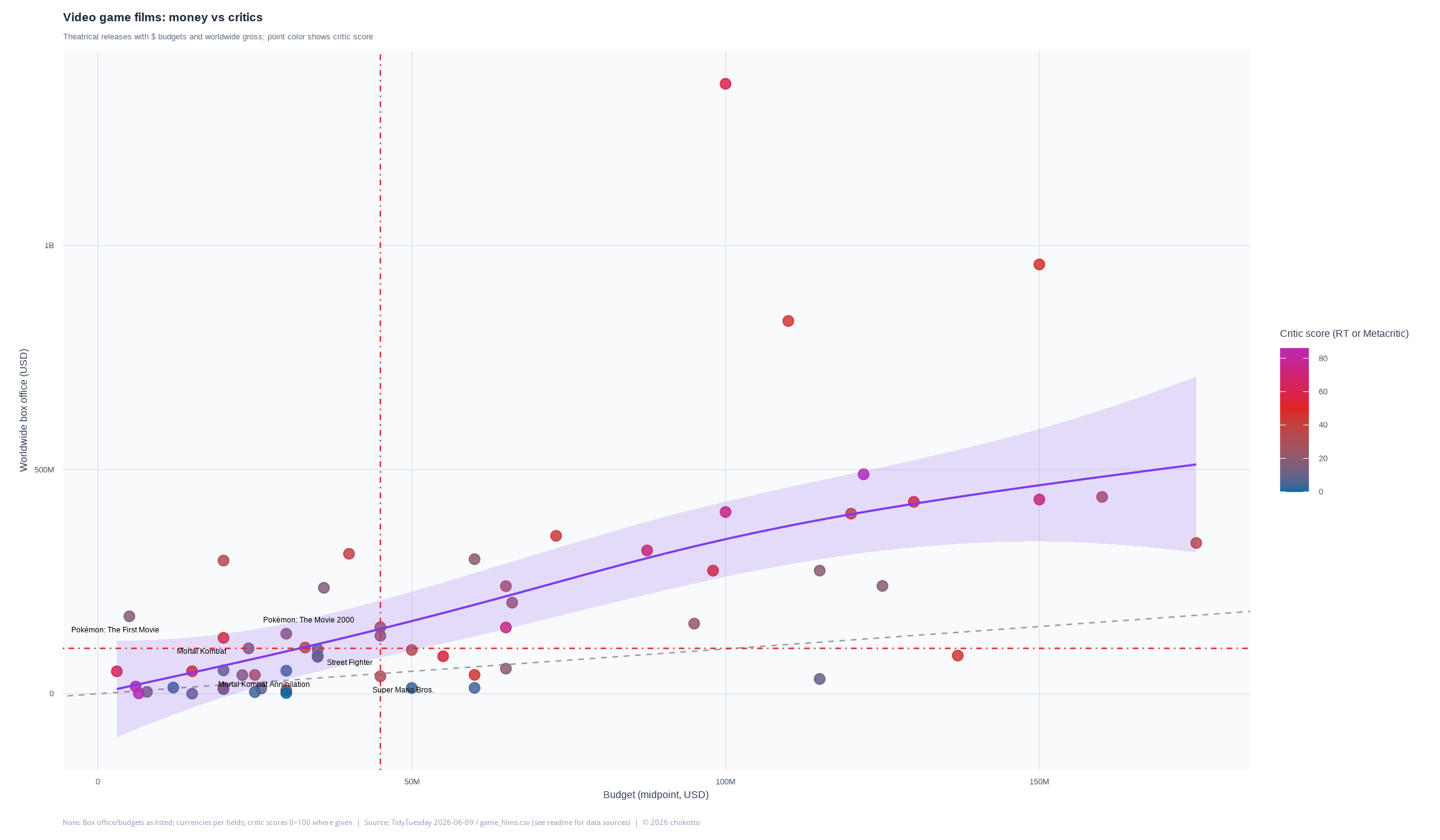
I’ll parse dates, extract years, and filter to category == “Theatrical releases”. Where budget_low and budget_high exist in dollars, I’ll take their midpoint and compare it to worldwide_box_office to sketch ROI. Because currencies aren’t harmonized, I’ll limit the core scatterplot to entries with $ in both budget_currency and worldwide_box_office_currency. I’ll layer critic sentiment (Rotten Tomatoes or Metacritic) as color, label a few well-known titles from the 1990s, and summarize medians for context. Missingness and outliers will be highlighted with light jitter and marginal distributions.

Visualization

films <- read_csv("data/game_films.csv", show_col_types = FALSE)

# keep only theatrical releases with USD budgets and worldwide grosses; build a critic score
df <- films %>%
  filter(category == "Theatrical releases",
         budget_currency == "$",
         worldwide_box_office_currency == "$") %>%
  mutate(release_date_parsed = lubridate::ymd(release_date),
         year = lubridate::year(release_date_parsed),
         # midpoint when both lows/highs present; otherwise fall back to either side
         budget_mid = case_when(
           !is.na(budget_low) & !is.na(budget_high) ~ (budget_low + budget_high) / 2,
           !is.na(budget_low) ~ budget_low,
           !is.na(budget_high) ~ budget_high,
           TRUE ~ NA_real_
         ),
         critic_score = coalesce(rotten_tomatoes, metacritic)) %>%
  filter(!is.na(budget_mid), !is.na(worldwide_box_office), !is.na(critic_score))

# labels: top theatrical grosses from the 1990s to call out a few recognisable titles
labels_90s <- df %>%
  filter(!is.na(year), year >= 1990, year <= 1999) %>%
  arrange(desc(worldwide_box_office)) %>%
  slice_head(n = 6)

med_budget <- median(df$budget_mid, na.rm = TRUE)
med_world <- median(df$worldwide_box_office, na.rm = TRUE)

p <- ggplot(df, aes(x = budget_mid, y = worldwide_box_office, color = critic_score)) +
  # break-even line (box office == budget)
  geom_abline(intercept = 0, slope = 1, linetype = "dashed", color = "grey60", linewidth = 0.4) +
  geom_point(alpha = 0.85, size = 2.6) +
  geom_smooth(method = "gam", formula = y ~ s(x, bs = "cs"), se = TRUE,
              color = PAL[2], fill = PAL[2], alpha = 0.16, linewidth = 0.6) +
  # median guides for orientation
  geom_vline(xintercept = med_budget, linetype = "dotdash", color = PAL[4], linewidth = 0.4) +
  geom_hline(yintercept = med_world, linetype = "dotdash", color = PAL[4], linewidth = 0.4) +
  # callout a handful of 90s titles
  geom_text_repel(data = labels_90s,
                  inherit.aes = FALSE,
                  aes(x = budget_mid, y = worldwide_box_office, label = title),
                  size = 3.1, max.overlaps = 12, box.padding = 0.4, segment.alpha = 0.6) +
  scale_x_continuous(labels = label_number(scale_cut = cut_short_scale()),
                     name = "Budget (midpoint, USD)") +
  scale_y_continuous(labels = label_number(scale_cut = cut_short_scale()),
                     name = "Worldwide box office (USD)") +
  scale_color_gradient2(low = PAL[1], mid = PAL[4], high = PAL[8], midpoint = 50,
                        name = "Critic score (RT or Metacritic)") +
  labs(
    title = combined_title,
    subtitle = combined_subtitle,
    caption = SOURCE_CAPTION
  ) +
  theme_active

p

Key Findings

• Super Mario Bros. (1993) grossed $38,912,465 worldwide on a $42–48M budget; Rotten Tomatoes 29, Metacritic 35, CinemaScore B+.
• Mortal Kombat (1995) earned $124,742,000 worldwide vs a $20M budget; critics: RT 47, Metacritic 60, audience A-.
• Out of 439 entries, 96 have worldwide_box_office (median $84.4M; min $61.5k; max $5.02B); 73 RT scores (median 30) and 63 Metacritic (median 36).

---

This post is part of the TidyTuesday weekly data visualization project.

CautionDisclaimer

This analysis is for educational and practice purposes only. Data visualizations and interpretations are based on the provided dataset and may not represent complete or current information.